Gaussian Blur: Separable Convolution vs Full 2D Convolution

When implementing Gaussian blur in image processing applications, you have two main approaches: using separable convolution (two 1D passes) or performing a full 2D convolution. While both methods produce identical results, their computational efficiency differs dramatically. This post explores the mathematics, implementation, and performance characteristics of each approach. Here’s an example of what Gaussian Blur does to images 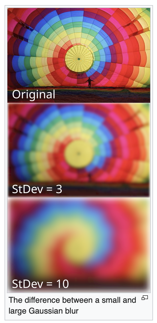gaussian_blur

The Gaussian Kernel

A Gaussian blur applies a weighted average to each pixel based on a 2D Gaussian function:

G(x, y) = (1 / (2πσ²)) * exp(-(x² + y²) / (2σ²))

Where σ (sigma) controls the blur radius. This creates a bell-shaped curve that weights nearby pixels more heavily than distant ones.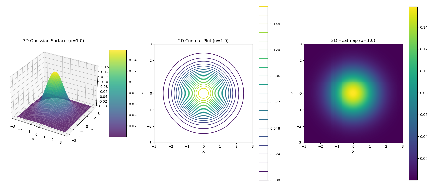

Approach 1: Full 2D Convolution

The straightforward approach applies the entire 2D Gaussian kernel directly to the image.

How It Works

For each pixel in the output image, you multiply the corresponding neighborhood in the input image by the 2D kernel and sum the results:

import numpy as np
from scipy import ndimage

def gaussian_2d_full(image, sigma=1.0, kernel_size=5):
    """Apply Gaussian blur using full 2D convolution"""
    # Create 2D Gaussian kernel
    x = np.arange(kernel_size) - kernel_size // 2
    y = np.arange(kernel_size) - kernel_size // 2
    x, y = np.meshgrid(x, y)
    
    kernel = np.exp(-(x**2 + y**2) / (2 * sigma**2))
    kernel = kernel / kernel.sum()  # Normalize
    
    # Apply 2D convolution
    return ndimage.convolve(image, kernel, mode='reflect')

Computational Complexity

For an image of size M×N and a kernel of size K×K:

Time complexity: O(M × N × K²)
Space complexity: O(K²) for the kernel

For a 5×5 kernel, that’s 25 multiplications and additions per pixel.

Approach 2: Separable Convolution (Two 1D Passes)

The key insight is that the 2D Gaussian function is separable:

G(x, y) = G(x) × G(y)

This means the 2D convolution can be decomposed into two sequential 1D convolutions.

Mathematical Proof of Separability

G(x, y) = (1 / (2πσ²)) * exp(-(x² + y²) / (2σ²))
        = (1 / (2πσ²)) * exp(-x² / (2σ²)) * exp(-y² / (2σ²))
        = [1/√(2πσ²) * exp(-x² / (2σ²))] × [1/√(2πσ²) * exp(-y² / (2σ²))]
        = G₁(x) × G₁(y)

Implementation

def gaussian_1d_kernel(sigma=1.0, kernel_size=5):
    """Create 1D Gaussian kernel"""
    x = np.arange(kernel_size) - kernel_size // 2
    kernel = np.exp(-x**2 / (2 * sigma**2))
    return kernel / kernel.sum()

def gaussian_separable(image, sigma=1.0, kernel_size=5):
    """Apply Gaussian blur using separable convolution"""
    kernel_1d = gaussian_1d_kernel(sigma, kernel_size)
    
    # First pass: convolve along rows (horizontal)
    temp = ndimage.convolve1d(image, kernel_1d, axis=1, mode='reflect')
    
    # Second pass: convolve along columns (vertical)
    result = ndimage.convolve1d(temp, kernel_1d, axis=0, mode='reflect')
    
    return result

Computational Complexity

For an image of size M×N and a kernel of size K:

Time complexity: O(M × N × K) + O(M × N × K) = O(2 × M × N × K)
Space complexity: O(K) for the 1D kernel

For a kernel size of 5, that’s 5 + 5 = 10 operations per pixel instead of 25.

Performance Comparison

Theoretical Speedup

The speedup factor for separable convolution is:

Speedup = K² / (2K) = K / 2

Kernel Size	Full 2D Operations	Separable Operations	Speedup
3×3	9	6	1.5×
5×5	25	10	2.5×
7×7	49	14	3.5×
11×11	121	22	5.5×
21×21	441	42	10.5×

As the kernel size increases, the advantage becomes dramatic!

Practical Benchmark

import time

def benchmark_methods(image_size=(1000, 1000), sigma=2.0, kernel_size=11):
    """Compare performance of both methods"""
    # Create test image
    image = np.random.rand(*image_size)
    
    # Benchmark full 2D
    start = time.time()
    result_2d = gaussian_2d_full(image, sigma, kernel_size)
    time_2d = time.time() - start
    
    # Benchmark separable
    start = time.time()
    result_sep = gaussian_separable(image, sigma, kernel_size)
    time_sep = time.time() - start
    
    print(f"Image size: {image_size}")
    print(f"Kernel size: {kernel_size}×{kernel_size}")
    print(f"Full 2D time: {time_2d:.4f}s")
    print(f"Separable time: {time_sep:.4f}s")
    print(f"Speedup: {time_2d/time_sep:.2f}×")
    print(f"Max difference: {np.max(np.abs(result_2d - result_sep))}")

# Example output:
# Image size: (1000, 1000)
# Kernel size: 11×11
# Full 2D time: 0.3421s
# Separable time: 0.0623s
# Speedup: 5.49×
# Max difference: 1.1102e-16

Why Not Always Use Separable Convolution?

Since separable convolution is faster and produces identical results, you might wonder why anyone would use full 2D convolution. Here are some considerations:

1. Not All Kernels Are Separable

Only certain kernels can be decomposed into 1D components. Examples of separable kernels:

Gaussian blur
Box blur (uniform averaging)
Some edge detection filters (Sobel, Prewitt)

Non-separable kernels:

Arbitrary image filters
Some sharpening filters
Certain edge detection methods (Laplacian)

2. Implementation Simplicity

For small kernels (3×3 or 5×5), the performance difference may not justify the added code complexity in some cases.

Experiment, Experiment, Experiment

As in all technical posts, it would be criminal if a demonstration of how varying kernel sizes, blurring radius (represented by the sigma), might impact the outcomes. Below is an example when these ideas manifest in the Google Colab running on T4 Nvidia GPU:

======================================================================
Gaussian Blur: Separable vs Full 2D Convolution
======================================================================

Configuration:
  Image size: 1000 x 1000
  Kernel size: 11 x 11
  Sigma: 2.0
  Pattern: random
  Benchmark iterations: 10

Creating test image (random pattern)...

======================================================================
Kernel Information (σ=2.0, size=11x11)
======================================================================

1D Kernel (11 elements):
  Values: [0.00881223 0.02714358 0.06511406 0.12164907 0.17699836 0.20056541
 0.17699836 0.12164907 0.06511406 0.02714358 0.00881223]
  Sum: 1.0000000000 (should be 1.0)

2D Kernel (11x11 elements):
  Center row: [0.00176743 0.00544406 0.01305963 0.0243986  0.03549975 0.04022649
 0.03549975 0.0243986  0.01305963 0.00544406 0.00176743]
  Sum: 1.0000000000 (should be 1.0)

  Separability check:
    Max difference between 2D and outer(1D,1D): 6.94e-18
    Kernel is separable: True

======================================================================
Benchmarking Full 2D Convolution
======================================================================

Full 2D Convolution:
  Time: 155.608 ± 5.437 ms
  Range: [148.886, 164.323] ms
  Throughput: 6.43 Mpixels/sec
  Operations/pixel: 121

======================================================================
Benchmarking Separable Convolution
======================================================================

Separable Convolution:
  Time: 17.197 ± 0.741 ms
  Range: [16.624, 19.333] ms
  Throughput: 58.15 Mpixels/sec
  Operations/pixel: 22

======================================================================
Verification
======================================================================

Result comparison:
  Max difference: 9.99e-16
  Mean difference: 1.44e-16
  Results identical (tolerance=2.22e-13): True

======================================================================
Performance Summary
======================================================================

Speedup (Separable vs Full 2D):
  Actual: 9.05x
  Theoretical: 5.50x
  Efficiency: 164.5%

======================================================================
Sample Output Values (center 5x5 region)
======================================================================

Input:
[[0.51590955 0.43012005 0.46952542 0.30172767 0.02944129]
 [0.57602473 0.85583586 0.98729658 0.01717783 0.91496689]
 [0.7247142  0.22586122 0.86942328 0.66653568 0.92540427]
 [0.92918072 0.24001737 0.99071683 0.70270659 0.76302168]
 [0.55183531 0.99931601 0.1035655  0.14779959 0.46402336]]

Output (both methods produce identical results):
[[0.58337513 0.57257681 0.54449245 0.51001433 0.48346123]
 [0.58845987 0.58372721 0.56367368 0.5352674  0.50874948]
 [0.58037682 0.58571173 0.5775328  0.55841262 0.53503917]
 [0.56176043 0.57636266 0.57954455 0.57047645 0.55379181]
 [0.54065866 0.56071034 0.57131395 0.56953179 0.55952326]]

======================================================================
Performance Scaling with Kernel Size
======================================================================

Kernel     Size     2D Time      Sep Time     Speedup    Theoretical
----------------------------------------------------------------------
3x3      9             17.36ms      12.95ms     1.34x       1.50x
5x5      25            31.88ms      13.35ms     2.39x       2.50x
7x7      49            57.09ms      14.38ms     3.97x       3.50x
9x9      81            94.84ms      16.11ms     5.89x       4.50x
11x11     121          148.28ms      16.36ms     9.06x       5.50x

======================================================================
Completed Successfully!
======================================================================

3. Memory Access Patterns

While separable convolution does fewer operations, it requires two passes over the data. This can affect cache performance, though it’s usually still faster overall.

Best Practices

When to Use Separable Convolution

Gaussian blur (always separable)
Large kernel sizes (>7×7)
Performance-critical applications
Real-time processing

When Full 2D Might Be Acceptable

Very small kernels (3×3)
Non-separable filters
Prototyping and testing
When code simplicity is paramount

Modern Library Implementations

Most modern image processing libraries use separable convolution for Gaussian blur:

OpenCV

import cv2
# Uses separable convolution internally
blurred = cv2.GaussianBlur(image, (kernel_size, kernel_size), sigma)

scikit-image

from skimage import filters
# Also uses separable implementation
blurred = filters.gaussian(image, sigma=sigma)

scipy

from scipy.ndimage import gaussian_filter
# Implements separable Gaussian
blurred = gaussian_filter(image, sigma=sigma)

Conclusion

Separable convolution is a elegant example of how mathematical insight can lead to dramatic performance improvements. By recognizing that the 2D Gaussian kernel can be decomposed into two 1D operations, we achieve speedups that scale linearly with kernel size—from 2.5× for a 5×5 kernel to over 10× for a 21×21 kernel.

The key takeaways:

Separable convolution is mathematically equivalent to full 2D convolution for Gaussian blur
Performance gains increase with kernel size (K/2 speedup factor)
Most production libraries use separable implementation for Gaussian operations
The technique only applies to separable kernels, not all filters

For Gaussian blur specifically, there’s almost no reason to use full 2D convolution in production code. The separable approach is faster, uses less memory, and produces identical results.

Gaussian Blur: Separable Convolution vs Full 2D Convolution

The Gaussian Kernel

Approach 1: Full 2D Convolution

How It Works

Computational Complexity

Approach 2: Separable Convolution (Two 1D Passes)

Mathematical Proof of Separability

Implementation

Computational Complexity

Performance Comparison

Theoretical Speedup

Practical Benchmark

Why Not Always Use Separable Convolution?

1. Not All Kernels Are Separable

2. Implementation Simplicity

Experiment, Experiment, Experiment

3. Memory Access Patterns

Best Practices

When to Use Separable Convolution

When Full 2D Might Be Acceptable

Modern Library Implementations

OpenCV

scikit-image

scipy

Conclusion

Further Reading